This page makes use of JavaScript.
My code is 100% nice: No external code, no trackers.
Enabling scripts for this document is recommended.
Algebraic Definition |
Geometric Definition |
| a · b = n i=1 aibi = a1b1 + a2b2 + ... anbn | a · b = |a| |b| cos θ |
The dot product tells us, how much one vector projects onto another. It is a measure, how similar the direction of a is to the normal vector of b. (In 3D, it compares to the normal plane of b.) For unit vectors, it ranges from -1 to +1, where +1 would indicate both vectors pointing in the same direction. This can be used to determine, if a face is pointing towards or away from the camera. For convex objects, only faces pointing to the camera need to be rendered, because faces seen from their back are obscured anyways.
cos θ = a · b |a| |b| = axbx + ayby ax2 + ay2 · bx2 + by2
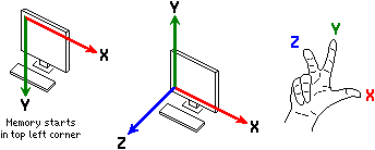
Computer hardware does not know about multi-dimensional arrays, or even more sophisticated data structures. Memory is ever only accessed via the addresses of each byte. Your programming language takes care of translating high level representations of data structures, like arrays, structs or objects, into physical memory addresses.
There are two ways, how a matrix can be stored in memory:
Matrix in row major order R =
r11
r12
r13
r21
r22
r23
r31
r32
r33
= Array(
r11,
r12,
r13,
r21,
r22,
r23,
r31,
r32,
r33
),
Matrix in column major order C =
c11
c21
c31
c12
c22
c32
c13
c23
c33
= Array(
c11,
c12,
c13,
c21,
c22,
c23,
c31,
c32,
c33
).
Obviously, it is important to know, which major order your system expects.
M = [xAxisx, xAxisy, xAxisz, 0,
     yAxisx, yAxisy, yAxisz, 0,
     zAxisx, zazisy, xAxisz, 0,
     Transx, Transy, Transz, 1];
According to Wikipedia, OpenGL uses vector-major order
(M[vector][coordinate] or M[column][row] respectively), which confuses me
somewhat. Further investigation is needed.
Calculating the determinant of a 2 × 2 or 3 × 3 matrix is fairly straight forward. An easy to remember rule is to add the products following the diagonals from top left to bottom right (while wrapping around the edges), and subtracting the products of the diagonals going from top right to bottom left, like so:
|M3| = det abc def ghi = aei + bfg + cdh - ceg - bdi - afh,
and for a 2 × 2 matrix:
|M2| = det ab cd = ad - bc.
The process for larger matrices is not as easily expressed by a simple rule; It involves recursively partitioning the matrix into smaller sub-matrices, whose determinants can be calculated like shown above. Check the Wikipedia article for details.
Still, solving equation systems with the Cramer Rule follows the same same pattern of dividing the determinants.
You have probably seen a linear equation before:
A general system of m linear equations with n unknowns can be written as:
The Cramer Rule is a method of solving such an equation system, which is very easy to code. It uses several sets of matrices, containing the coeficcients of the equations. The basic matrix M looks like so:
M = a11 a12 ⋯ a1n a21 a22 ⋯ a2n ⋮ ⋮ ⋱ ⋮ am1 am2 ⋯ amn .
Note, that we did not include the constant offsets bm in this matrix.
We need another matrix for each of the unknowns, where the coefficients amn for the unknown is replaced with the offset bm. Let's assume a system of 3 equations with 3 unknowns, x, y, and z, for easier demonstration:
Our base matrix M and substituted matrices Mx, My and Mz are:
M = A1 B1 C1 A2 B2 C2 A3 B3 C3 , Mx = D1 B1 C1 D2 B2 C2 D3 B3 C3 , My = A1 D1 C1 A2 D2 C2 A3 D3 C3 , Mz = A1 B1 D1 A2 B2 D2 A3 B3 D3 .
Then, we get the solutions for our equation system by simply dividing the determinants of the matrices:
x = |Mx||M|, y = |My||M|, and z = |Mz||M|.
Since a vector is essentially a matrix with only one element per row, the process of matrix-vector multiplication is rather simple; One takes the dot product of x with each row of A:
Ax = a11 a12 ⋯ a1n a21 a22 ⋯ a2n ⋮ ⋮ ⋱ ⋮ am1 am2 ⋯ amn x1 x2 ⋮ xn = a11x1 + a12x2 + ⋯ + a1nxn a21x1 + a22x2 + ⋯ + a2nxn ⋮ am1x1 + am2x2 + ⋯ + amnxn
If A = 1-12 0-31 , x = 210 , then Ax = 1·2 - 1·1 + 2·0 0·2 - 3·1 + 1·0 = 1 -3
If A is an m × n matrix, and B is an n × p matrix, A = a11 a12 ⋯ a1n a21 a22 ⋯ a2n ⋮ ⋮ ⋱ ⋮ am1 am2 ⋯ amn , B = b11 b12 ⋯ b1p b21 b22 ⋯ b2p ⋮ ⋮ ⋱ ⋮ bn1 bn2 ⋯ bnp , the matrix product C = AB is defined to be the m × p matrix C = AB = c11 c12 ⋯ c1p c21 c22 ⋯ c2p ⋮ ⋮ ⋱ ⋮ cm1 cm2 ⋯ cmp , where cij = ai1b1j + ai2b2j + ... + ainbnj = n k=1 aikbkj, for i = 1, ..., m and j = 1, ..., p.
That is, the entry cij of the product is obtained by multiplying term-by-term the entries of the ith row of A and the jth column of B, and summing these n products. In other words, cij is the dot product of the ith row of A and the jth column of B.
Therefore, AB can also be written as C = a11b11 + ⋯ + a1nbn1 a11b12 + ⋯ + a1nbn2 ⋯ a11b1p + ⋯ + a1nbnp a21b11 + ⋯ + a2nbn1 a21b12 + ⋯ + a2nbn2 ⋯ a21b1p + ⋯ + a2nbnp ⋮ ⋮ ⋱ ⋮ am1b11 + ⋯ + amnbn1 am1b12 + ⋯ + amnbn2 ⋯ am1b1p + ⋯ + amnbnp
Thus the product AB is defined if and only if the number of columns in A equals the number of rows in B, in this case n.
A = a11 a12 a13 a21 a22 a23 a31 a32 a23 , B = b11 b12 b13 b11 b22 b23 b11 b22 b23 , AB = a11b11 + a12b21 + a13b31 a11b12 + a12b22 + a13b32 a11b13 + a12b23 + a13b33 a21b11 + a22b21 + a23b31 a21b12 + a22b22 + a23b32 a21b13 + a22b23 + a23b33 a31b11 + a32b21 + a33b31 a31b12 + a32b22 + a33b32 a31b13 + a32b23 + a33b33 .
C2 × 2 = A2 × 3B3 × 2 = a11 a12 a13 a11 a22 a23 b11 b12 b21 b22 b31 b32 , where n = 3, m = p = 2; C = AB = a11b11 + a12b21 + a13b31 a11b12 + a12b22 + a13b32 a21b11 + a22b21 + a23b31 a21b12 + a22b22 + a23b32 .
For practical reasons, 4 × 4 matrices are used with 3D graphics. For details, see the section about Transformation Matrices.
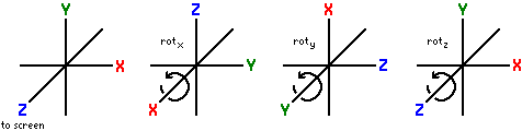
rotation_x_mat4()
rotation_y_mat4()
rotation_z_mat4()
function on_update_scene (elapsed_seconds) {
	const angle = 60*DtoR * elapsed_seconds;
	VMath.mat4_multiply_mat4(
		entity.rotation_matrix,
		entity.rotation_matrix,
		VMath.rotation_<axis>_mat4( angle ),
	);
}
X = rotx θ = 1 0 0 0 0 cos θ -sin θ 0 0 sin θ cos θ 0 0 0 0 1 , Y = roty θ = cos θ 0 sin θ 0 0 1 0 0 -sin θ 0 cos θ 0 0 0 0 1 , Z = rotz θ = cos θ -sin θ 0 0 sin θ cos θ 0 0 0 0 1 0 0 0 0 1 .
Thus, a = xyz1 ≘ x 0 0 0 0 y 0 0 0 0 z 0 0 0 0 1 , a' = aX = x y cos θ - z sin θ y sin θ + z cos θ 1 .
n = nx ny nz , Mrot n = tnx2+c tnxny-snz tnxnz+sny 0 tnxny+snz tny2+c tnynz-snx 0 tnxnz-sny tnynz+snx tnz2+c 0 0 0 0 1 , where s = sin θ, c = cos θ and t = 1 - cos θ.